Getting started with keras in R

The RStudio produced package for keras was the subject of the keynote at this year's rstudio-conf.
Keras is a python API designed to provide a higher level interface to the neural network backends Tensorflow, CNTK and Theano. The most common of these is Tensorflow and that is the one we will use as well. In this post I'll outline the steps I took to get some hello world models up and running in R and also some of the nice additional things you can do with the new R packages.
I won't go into too much detail about the background of keras, mainly because the existing documentation is very good:
- RStudio / keras reference: https://tensorflow.rstudio.com
- Keras documentation (for more details on options and explanations): https://keras.io/
I also won't go into too much detail about the nuts and bolts of deep learning because there are some fantastic resources that are only a google away. If you want a great introduction, go and watch Andrew Ng's youtube course (don't worry, we'll wait for you).
The set up
You need a machine with the tensorflow backend and you will also need python because the R package accesses the underlying python libraries (through a great little intermediate package called reticulate(https://github.com/rstudio/reticulate)
You can use a CPU for computations, but if you have a CUDA enabled GPU it's worth installing the GPU variant of tensorflow because it is much faster.
Get the R libraries
The first thing you need to do is install the tensorflow R package. You can then use this to manage the install of the tensorflow back-end.
install.packages("tensorflow")
library(tensorflow)
I'd recommend the development version of keras for now because there are some fixes to line up the R package with the latest version of the keras python packages that it relies on.
devtools::install_github("rstudio/keras")The tfruns package is also very handy for recording and comparing model runs (we'll get to that in the next post).
CPU setup
The CPU setup is straightforward and can be done in R:
install_tensorflow()GPU requirements
My current set up is a NVIDA GTX1080 machine powered by ubuntu 16.04. It takes some care to ensure all your library and driver versions match. At time of writing I would recommend CUDA toolkit v9.0, cuDNN (the deep neural network library) 7.0 and tensorflow 1.5.
Then you have a one-line install in R
install_tensorflow(tensorflow = "gpu")Why am I so sure about that recommendation? Because I installed CUDA toolkit version 9.1 which is not supported by the prebuilt tensorflow binaries, so I lost an hour or so compiling tensorflow from source. Everything worked fine after that though.
If you do run into trouble with configurations (or python version conflicts) you can easily check your configuration with
reticulate::py_discover_config("tensorflow")
reticulate::py_discover_config("keras")
The fun stuff
We will start with the MNIST handwriting dataset, because what the internet needs right now is another MNIST example, amiright?
First, get the MNIST data (it's included with the package)
library(keras)
library(tensorflow)
library(imager)  # very helpful image package

mnist <- dataset_mnist()
x_train <- mnist$train$x
y_train <- mnist$train$y

x_test <- mnist$test$x
y_test <- mnist$test$y

dim(x_train)
dim(y_train)
The training set is an array class and contains 60000 28 x 28 image arrays. Here's a sample:
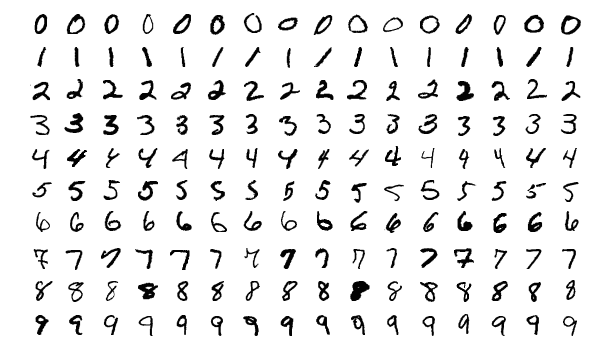
By Josef Steppan via Wikimedia Commons
Step one - deep neural net
Tensorflow requires the data with dimensions [ No_images rows X 784 cols] (i.e. each row contains a vector of image pixels).
We also scale the data so each pixel value lies between 0 and 1.
x_train <- array_reshape(x_train, c(nrow(x_train), 784))
x_test <- array_reshape(x_test, c(nrow(x_test), 784))
x_train <- x_train / 255
x_test <- x_test / 255

dim(x_train)
We need to make the response data categorical. The function keras::to_categorical Converts a vector of integers to binary data in a matrix. In this case we convert y_train from integer classes between 0 and 9 to a binary matrix (0's and 1's in an [NIMG x 10] dimensional array).
Note: this step is necessary because we are using the
categorical_crossentropyloss function in the model below. This note explains it (https://keras.io/losses/#usage-of-loss-functions) :
head(y_train)
y_train <- to_categorical(y_train, 10)
y_test <- to_categorical(y_test, 10)
head(y_train)
About the models
Keras/TF use symbolic computation so we need to set up the model graph first. The keras libary has a bunch of different layer types you can use.
The model itself will probably be initialised using keras::keras_model_sequential which is just a linear stack of layers. The multi_gpu_model function allows you to initalise the model over multiple gpus (but you probably already guessed that).
Useful layer types:
layer_dense()A fully/densely connected layer. Useful settings areactivation,use_bias,kernel_initializer,weights(allows you to initialise the kernel weights and layer weights),kernel_regularizer,units(dimensions of the output space).
layer_activation(activation = "name")adds an activition layer (or if it's one of the standard ones you can do it in thelayer_denseorlayer_conv_Xcalls). See https://keras.io/activations/ for list of basics.layer_activation_leaky_reluadds a leaky relu activation specifically.layer_dropout()adds a dropout.rateis number between 0 and 1 that specifies the fraction to drop out.layer_flatten()flattens the layer (e.g. going from convolution cycle to fully connected layers).
There are also a bunch of options for convolutions and for pooling layers. layer_conv_2d and layer_max_pooling_2d are two of the most common ones.
First define a model
Let's define a really simple model, with one dense (fully connected) layer, a dropout layer and a final softmax
model <- keras_model_sequential()
model %>%
  layer_dense(units = 256, activation = 'relu',  input_shape = c(784)) %>%
  layer_dropout(rate = 0.4) %>% layer_dense(units = 128, activation = 'relu') %>%
  layer_dense(units = 10, activation = 'softmax')
summary(model)
One nice feature of the keras package is the model detail you get when you run summary - very handy to enable quick and dirty calculations to see if your next model run is going to blow smoke out of the GPU...

Compile the model
The compilation stage is where you define the hyperparameters, .e.g.
- loss functions - You can use any of the keras library so see https://keras.io/losses/#available-loss-functions
- opimizer - again, see https://keras.io/optimizers/
- Metrics - track ALL THE THINGS: https://keras.io/metrics/
We are using categorical_crossentropy loss function (link).
# compile (define loss and optimizer)
model %>% keras::compile(
  loss = 'categorical_crossentropy',
  optimizer = optimizer_rmsprop(),
  metrics = c('accuracy')
  )
Fit the model and test
Finally, at runtime we set the number of epochs, the batch size and validation split (what percentage of the training data will be kept aside for validation).
# train (fit)
model %>% fit(
  x_train,
  y_train,
  epochs = 15,
  batch_size = 128,
  validation_split = 0.2,
  verbose = 1
)
Another nice feature of the keras library (as opposed to, say the mxnet library) is tracking the loss function and accuracy as the model is training (see the clip above)
By the end of the training run our model accuracy on the training set is around 98.51% on the training set and 97.95% on the validation set. It's possible to get a higher accuracy than this, but I'll leave that exploration up to you readers (feel free to share your experiments in the comments).
With 98% accuracy our model is fairly well optimised (for a first go). But having an optimised model (i.e. a good performance on the training set) is not the same as having a generalised model. We need to ensure we have not overfit the model by testing the prediction accuracy against our test set.
This is also straightforward:
model %>%
  evaluate(x_test, y_test)
We get a prediction accuracy of 98.06% on the test set. Again, this is pretty good for a hello world.
What's next?
At Symbolix we will be using more of R/keras for our machine and deep learning analysis (we are quite impressed). I am hoping to write more of these walkthroughs - what would you like to see next?